transformBarycentric

Conversion to barycentric coordinates

Converts the expression matrix containing three biological conditions to barycentric coordinates, reducing its dimensionality by one while retaining information of differential expression.

Usage

transformBarycentric(E, transfomatrix = NULL)

Arguments

E

Expression matrix

transfomatrix

NULL (default) or a numeric matrix containing the transformation matrix

Value

Dataframe containing for every original point its new coordinates in d-1 dimensions

Examples

Eoi = matrix(rnorm(1000*3, sd=0.5), 1000, 3, dimnames=list(1:1000, c(1,2,3)))
Eoi[1:100,1] = Eoi[1:100,1] + 1
barycoords = transformBarycentric(Eoi)
hist(barycoords$angle)

transformReverseBarycentric

Convert from barycentric coordinates back to original expression values

Converts a dataframe contain barycentric coordinates in the x and y columns back to original coordinates (apart from a constant for each gene).

Usage

transformReverseBarycentric(barycoords, transfomatrix = NULL)

Arguments

barycoords

Dataframe of barycentric coordinates with x and y in separate columns

transfomatrix

NULL (default) or a numeric matrix containing the transformation matrix

Value

Matrix containing for every gene original expression values centered around 0

Examples

Eoi = matrix(rnorm(1000*3, sd=0.5), 1000, 3, dimnames=list(1:1000, c(1,2,3)))
Eoi[1:100,1] = Eoi[1:100,1] + 1
barycoords = transformBarycentric(Eoi)
reversebarycoords = transformReverseBarycentric(barycoords)
all.equal(scale(t(Eoi)), scale(t(reversebarycoords)), check.attributes=FALSE)

## [1] TRUE

getTransformationMatrix

Barycentric transformation matrix

Get the matrix for the barycentric transformation

Usage

getTransformationMatrix(anglebase = 0)

Arguments

anglebase

Number of radians the first barycentric direction should be rotated anticlockwise

Value

2 by 3 matrix

Examples

plot(t(getTransformationMatrix(0)), asp=1)

plot(t(getTransformationMatrix(pi/2)), asp=1)

plot(t(getTransformationMatrix(pi)), asp=1)

plotDotplot

Creating a dotplot

Plot a dotplot

Usage

plotDotplot(barycoords, Gdiffexp = rownames(barycoords), Goi = NULL, Coi = attr(barycoords, "conditions"), colorby = "diffexp", colorvalues = NULL, rmax = 5, showlabels = TRUE, sizevalues = stats::setNames(c(0.5, 2), c(FALSE, TRUE)), alphavalues = stats::setNames(c(0.8, 0.8), c(FALSE, TRUE)), barycoords2 = NULL, baseangle = 0)

Arguments

barycoords

Dataframe containing for every gene its barycentric coordinates, as returned by transformBarycentric

Gdiffexp

Differentially expressed genes

Goi

Genes of interest, a character or numeric vector to plot one set of genes, a named list containing different such vectors to plot multiple gene sets

Coi

Character vector specifying the names of the three biological conditions, used for labelling

colorby

Color by differential expression (“diffexp”) or by log fold-change (“z”)

colorvalues

Color values, different syntax depending on the colorby parameter:

• diffexp: Named list with colors. First part of the name denotes whether a gene is differentially expressed (diffexp or nodiffexp). The second part denotes the name of the gene set. Genes not within a gene set are denoted by all. For example: list(diffexpall=“#000000”, nodiffexpall=“#AAAAAA”, nodiffexpgset=“#FFAAAA”, diffexpgset=“#FF0000”)
• z: A character vector of color values, used to generate the color gradient

rmax

Number denoting the maximal radius of the grid. All points outside of the grid will be clipped on the boundaries.

showlabels

Whether to show labels on the grid

sizevalues

Named list with the size of each dot if differentially expressed (TRUE) or not (FALSE)

alphavalues

Named list with the alpha value of each dot if differentially expressed (TRUE) or not (FALSE)

barycoords2

Dataframe containing for every gene a second set of barycentric coordinates, as returned by transformBarycentric. An arrow will be drawn from the coordinates in barycoords to those in barycoords2

baseangle

The angle by which to rotate the whole plot (default to 0)

Value

A ggplot2 plot, which can be used for further customization

Examples

data(vandelaar)
Eoi <- limma::avearrays(vandelaar, Biobase::phenoData(vandelaar)$celltype)
Eoi = Eoi[,c("YS_MF", "FL_mono", "BM_mono")]
barycoords = transformBarycentric(Eoi)
plotDotplot(barycoords)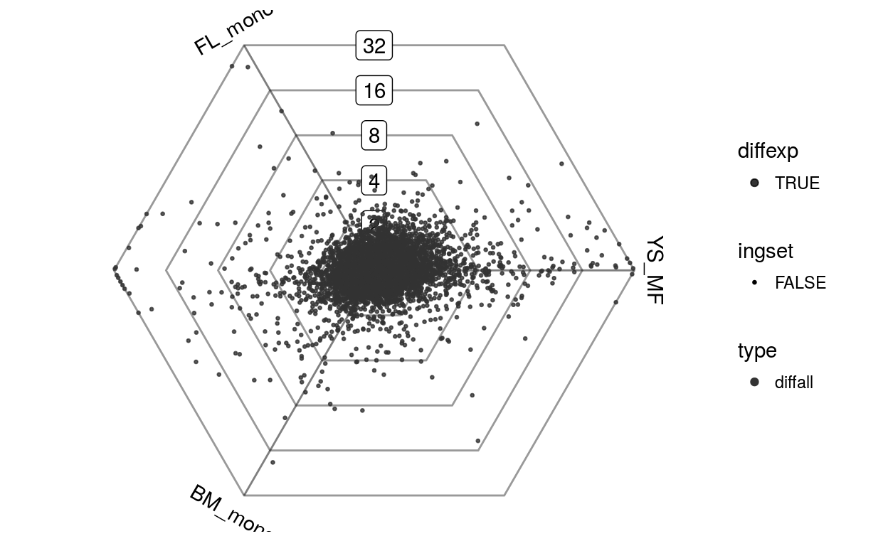

Eoi = matrix(rnorm(1000*3, sd=0.5), 1000, 3, dimnames=list(1:1000, c(1,2,3)))
Eoi[1:100,1] = Eoi[1:100,1] + 1
barycoords = transformBarycentric(Eoi)
Gdiffexp =(1:1000)[barycoords$r > 1]
plotDotplot(barycoords)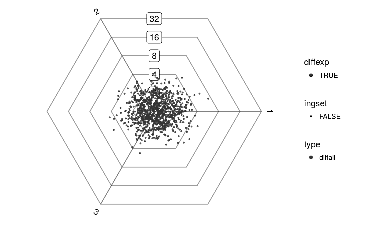

plotDotplot(barycoords, Gdiffexp)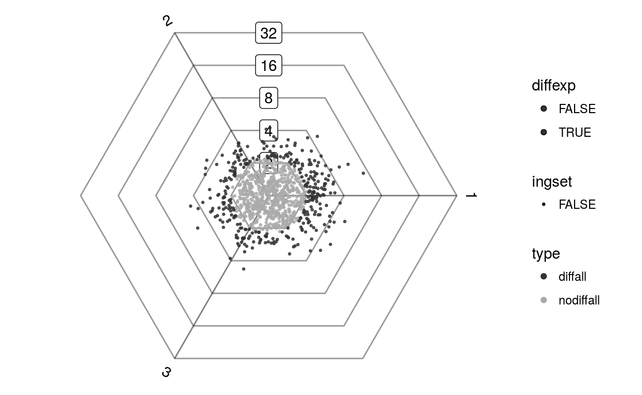

plotDotplot(barycoords, Gdiffexp, 1:100)

plotDotplot(barycoords, Gdiffexp, list(a=1:100, b=sample(100:1000, 50)))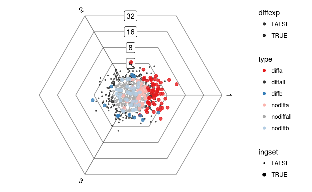

plotRoseplot

Plot the directional distribution of genes

A rose plot shows the distribution of a given set of genes in different directions.

Usage

plotRoseplot(barycoords, Gdiffexp = rownames(barycoords), Goi = rownames(barycoords), size = "surface", relative = TRUE, showlabels = TRUE, Coi = attr(barycoords, "conditions"), nbins = 12, bincolors = grDevices::rainbow(nbins, start = 0, v = 0.8, s = 0.6), rmax = "auto", baseangle = 0)

Arguments

barycoords

Dataframe containing barycentric coordinates as returned by transformBarycentric.

Gdiffexp

List of differentially expressed genes

Goi

List of genes of interest

size

Should the radius or the surface of a circle sector denote the number of genes differentially expressed in a particular direction

relative

Whether to show the relative number of genes or the absolute number of genes

showlabels

Whether to label the grid

Coi

Names of the three biological conditions, used for labelling

nbins

Number of bins, should be a multiple of 3 to make sense

bincolors

Colors of every bin, defaults to a rainbow palette

rmax

Number or “auto” (default), denotes the maximal radius of the grid.

baseangle

The angle by which to rotate the whole plot (default to 0)

Value

A ggplot2 plot, which can be used to further customize the plot

Examples

Eoi = matrix(rnorm(1000*3, sd=0.5), 1000, 3, dimnames=list(1:1000, c(1,2,3)))
Eoi[1:100,1] = Eoi[1:100,1] + 1
barycoords = transformBarycentric(Eoi)
plotRoseplot(barycoords)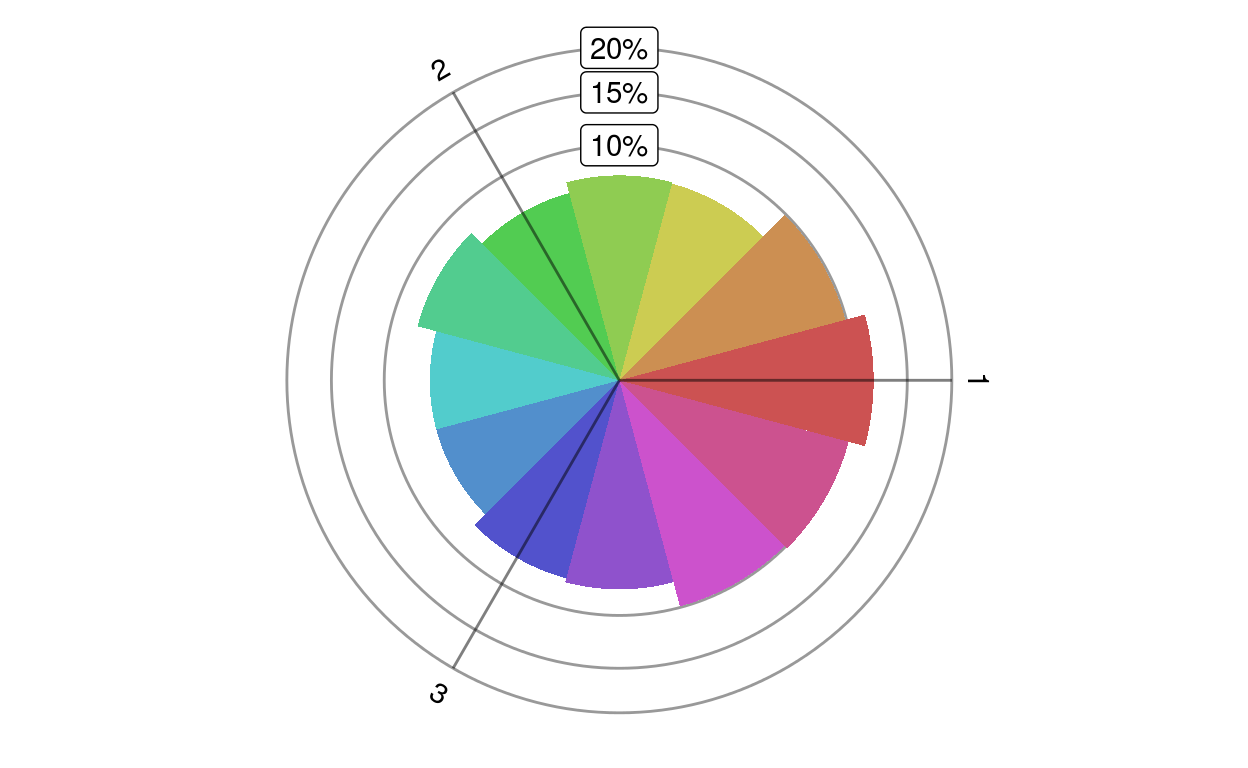

plotRoseplot(barycoords, (1:1000)[barycoords$r > 1])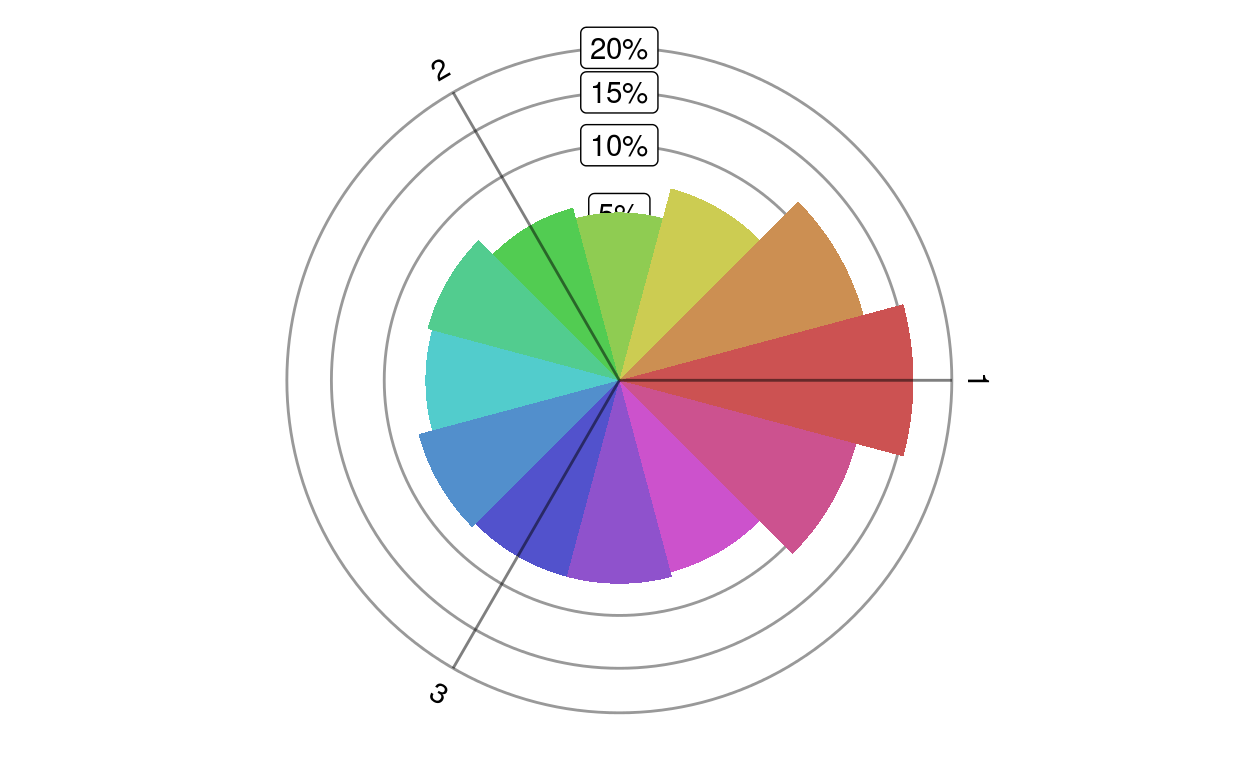

plotRoseplot(barycoords, (1:1000)[barycoords$r > 1], 1:100)

plotPvalplot

Plot results from unidirectional enrichment

Plots each enriched gene set as a dot on a dotplot

Usage

plotPvalplot(scores, Coi = c("", "", ""), colorby = NULL, showlabels = TRUE, baseangle = 0)

Arguments

scores

Dataframe as returned by testUnidirectionality containing for every gene set a q-value and an associated angle

Coi

Names of the three biological conditions, only used for labelling

colorby

Column in scores used for coloring

showlabels

Whether to show labels on the grid

baseangle

The angle by which to rotate the whole plot (default to 0)

Value

A ggplot2 plot, which can be used for further customization

Examples

Eoi = matrix(rnorm(1000*3, sd=0.5), 1000, 3, dimnames=list(1:1000, c(1,2,3)))
Eoi[1:100,1] = Eoi[1:100,1] + 4 # the first 100 genes are more upregulated in the first condition
barycoords = transformBarycentric(Eoi)

gsets = list(a=1:50, b=80:150, c=200:500)
scores = testUnidirectionality(barycoords, gsets, Gdiffexp=(1:1000)[barycoords$r > 1])

plotPvalplot(scores)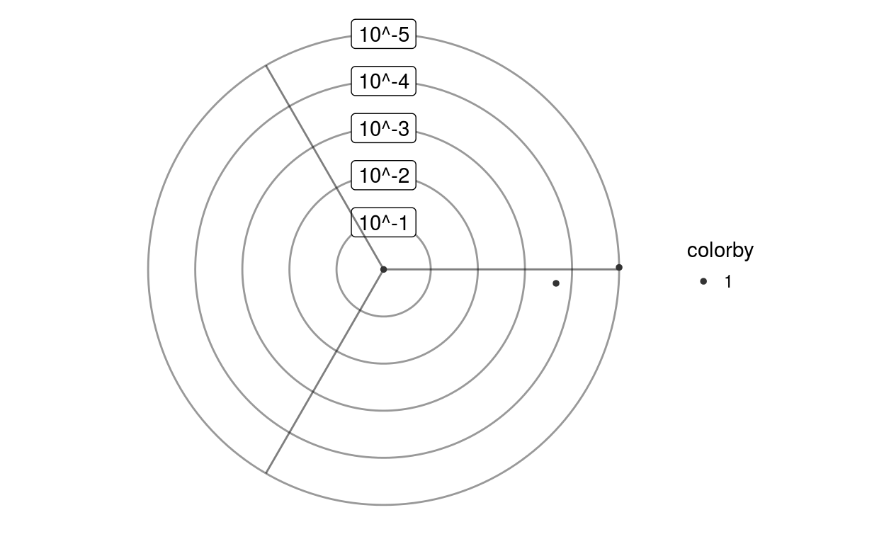

interactiveDotplot

Interactive triwise dotplot

Draw an interactive triwise dotplot using a html widget

Usage

interactiveDotplot(Eoi, Gdiffexp = rownames(Eoi), Goi = c(), Glabels = rownames(Eoi), Gpin = c(), Coi = colnames(Eoi), colorvalues = NULL, rmax = 5, sizevalues = c(`TRUE` = 2, `FALSE` = 0.5), alphavalues = c(`TRUE` = 0.8, `FALSE` = 0.8), plotLocalEnrichment = FALSE, width = NULL, height = NULL)

Arguments

Eoi

Expression matrix with the three conditions in the columns

Gdiffexp

Differentially expressed genes

Goi

Genes of interest, a character or numeric vector to plot one set of genes, a named list containing different such vectors to plot multiple gene sets

Glabels

Labels for every gene if different from the rownames of Eoi

Gpin

Pinned genes, if NULL will automatically choose the top 20 most differentially expressed genes

Coi

Character vector specifying the names of the three biological conditions, used for labelling

colorvalues

Color values, different syntax depending on the colorby parameter:

• diffexp: Named list with colors. First part of the name denotes whether a gene is differentially expressed (diffexp or nodiffexp). The second part denotes the name of the gene set. Genes not within a gene set are denoted by all. For example: list(diffexpall=“#000000”, nodiffexpall=“#AAAAAA”, nodiffexpgset=“#FFAAAA”, diffexpgset=“#FF0000”)
• z: A character vector of color values, used to generate the color gradient

rmax

Number denoting the maximal radius of the grid. All points outside of the grid will be clipped on the boundaries.

sizevalues

Named list with the size of each dot if differentially expressed (TRUE) or not (FALSE)

alphavalues

Named list with the alpha value of each dot if differentially expressed (TRUE) or not (FALSE)

plotLocalEnrichment

Whether to plot local enrichment as a ring around the dotplot

width

Width of the plot

height

Height of the plot

Value

A htmlwidget object, which can be exported to an svg using saveWidget

Examples

data(vandelaar)
Eoi <- limma::avearrays(vandelaar, Biobase::phenoData(vandelaar)$celltype)
Eoi = Eoi[,c("YS_MF", "FL_mono", "BM_mono")]
barycoords = transformBarycentric(Eoi)
## Not run: 
# interactiveDotplot(barycoords)
# ## End(Not run)

Eoi = matrix(rnorm(1000*3, sd=0.5), 1000, 3, dimnames=list(1:1000, c(1,2,3)))
Eoi[1:100,1] = Eoi[1:100,1] + 1
barycoords = transformBarycentric(Eoi)
Gdiffexp =(1:1000)[barycoords$r > 1]

## Not run: 
# interactiveDotplot(Eoi)
# interactiveDotplot(Eoi, Gdiffexp)
# interactiveDotplot(Eoi, as.character(Gdiffexp), as.character(1:10), as.character(1:1000))
# interactiveDotplot(Eoi, as.character(Gdiffexp), as.character(1:10), as.character(1:1000), c(50, 200))
# ## End(Not run)

interactivePvalplot

Interactive plot of p-values

Draw a dotplot of p-values using a htmlwidget

Usage

interactivePvalplot(scores, gsetlabels, Coi, width = NULL, height = NULL)

Arguments

scores

Dataframe as returned by testUnidirectionality containing for every gene set a q-value and an associated angle

gsetlabels

Names of the gene sets, used for hovering

Coi

Names of the three biological conditions, only used for labelling

width

Width of the plot

height

Height of the plot

Value

A htmlwidget object, which can be exported to an svg using saveWidget

Examples

Eoi = matrix(rnorm(1000*3, sd=0.5), 1000, 3, dimnames=list(1:1000, c(1,2,3)))
Eoi[1:100,1] = Eoi[1:100,1] + 4 # the first 100 genes are more upregulated in the first condition
barycoords = transformBarycentric(Eoi)

gsets = list(a=1:50, b=80:150, c=200:500)
scores = testUnidirectionality(barycoords, gsets, Gdiffexp=(1:1000)[barycoords$r > 1])
## Not run: 
# interactivePvalplot(scores, as.list(setNames(names(gsets), names(gsets))), 1:3)
# ## End(Not run)

testUnidirectionality

Test gene sets for unidirectional enrichment

Usage

testUnidirectionality(barycoords, gsets, Gdiffexp = NULL, statistic = "diffexp", bm = NULL, minknown = 5, mindiffexp = 0, maxknown = 1500, mc.cores = getOption("mc.cores", default = 1), ...)

Arguments

barycoords

Dataframe containing for every gene its barycentric coordinates, as returned by transformBarycentric

gsets

List of character vectors, each containing a set of genes (gene identifiers)

Gdiffexp

Differentially expressed genes

statistic

A string denoting the measure used for the strength of upregulation of a particular gene.

• diffexp: Whether a gene is differentially expressed (1 versus 0)
• rank: The rank of the maximal log fold-change
• r: The maximal log fold-change
• z: Custom using the z-column within barycoords
• angle: Uses a rayleigh z-test ignoring non-differentially expressed genes within the gene set

bm

Previously calculated background model using the generateBackgroundModel

minknown

Minimal number of genes within a gene set for it to be considered for enrichment

mindiffexp

Minimal number of genes differentially expressed within a gene set for it to be considered for enrichment

maxknown

Maximal number of genes within a gene set for it to be considered for enrichment

mc.cores

Number of processor cores to use. Due to limitations of the parallel package, this does not work on Windows

…

Parameters for generateBackgroundModel

Value

Dataframe containing for every gene set which passed the filtering:

• p-value of unidirectionality
• q-value of unidirectionality (p-value corrected for multiple testing)
• average angle

Examples

Eoi = matrix(rnorm(1000*3, sd=0.5), 1000, 3, dimnames=list(1:1000, c(1,2,3)))
Eoi[1:100,1] = Eoi[1:100,1] + 4 # the first 100 genes are more upregulated in the first condition
barycoords = transformBarycentric(Eoi)

gsets = list(a=1:50, b=80:150, c=200:500)
testUnidirectionality(barycoords, gsets, Gdiffexp=(1:1000)[barycoords$r > 1])

##           pval      angle   n gsetid          z         qval
## 1 0.0000000000 0.01545295  50      a 0.98546551 0.0000000000
## 2 0.0004658351 0.03248947  71      b 0.31799432 0.0006987526
## 3 0.9927447804 5.92573169 301      c 0.02986189 0.9927447804

generateBackgroundModel

Generate background models

Generates a background model by randomly resampling genes at different n (number of genes) and angles and calculating z distributions

Usage

generateBackgroundModel(barycoords, noi = seq(5, 100, 5), anglesoi = seqClosed(0, 2 * pi, 24), nsamples = 1e+05, bw = 20, mc.cores = getOption("mc.cores", default = 1))

Arguments

barycoords

Dataframe containing for every gene its barycentric coordinates, as returned by transformBarycentric. Will use the z column as test statistic, or if this column is not given the r column

noi

Integer vector denoting the number of genes at which to sample, the larger the more accurate the p-values

anglesoi

Numeric vector denoting the angles (in radians) at which to pre-calculate null distribution, the larger the more accurate the p-values

nsamples

Number of samples, higher for more accurate and stable p-values

bw

Bandwidth of the von-mises distribution for weighing the samples. A higher bandwidth leads to a more accurate p-value estimate as long as nsamples is high enough

mc.cores

Number of processor cores to use. Due to limitations of the parallel package, this does not work on Windows

Value

A list containing:

• noi: number of genes, in the same order as the elements in backmodels
• anglesoi: angles at which weights were calculated using the von-mises distribution
• nsamples: number of samples for each n
• bw: bandwidth
• backmodels: for each n a second list containing:
  • angles: mean angle of a sample
  • z: strength of unidirectional upregulation
  • weights: weight from von-mises distribution for every sample and angle in anglesoi, these weights will be used to calculate the p-value

Examples

Eoi = matrix(rnorm(1000*3, sd=0.5), 1000, 3, dimnames=list(1:1000, c(1,2,3)))
Eoi[1:100,1] = Eoi[1:100,1] + 1
barycoords = transformBarycentric(Eoi)

hist(barycoords$angle)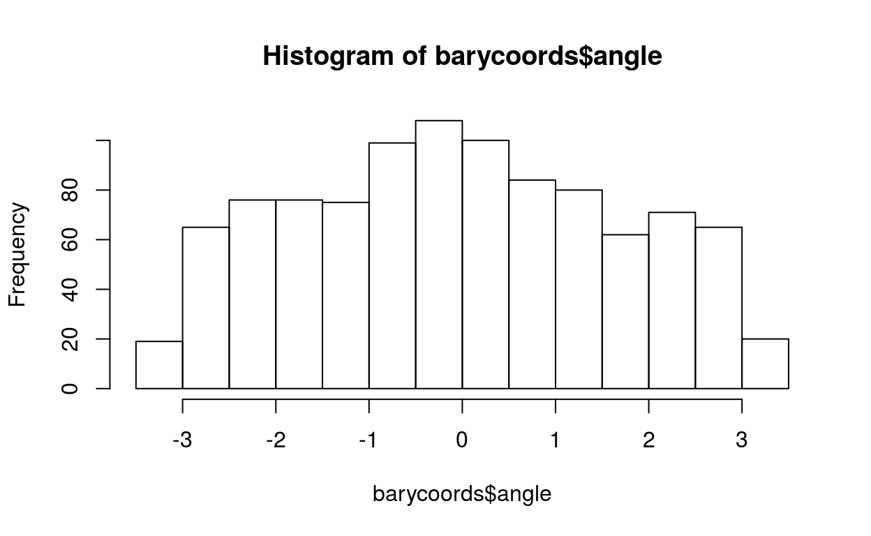

bm = generateBackgroundModel(barycoords)

# the distribution of mean angle of the samples is not uniform due to the non-uniform distribution of the angles of individual genes
hist(bm$backmodels[[1]]$angles)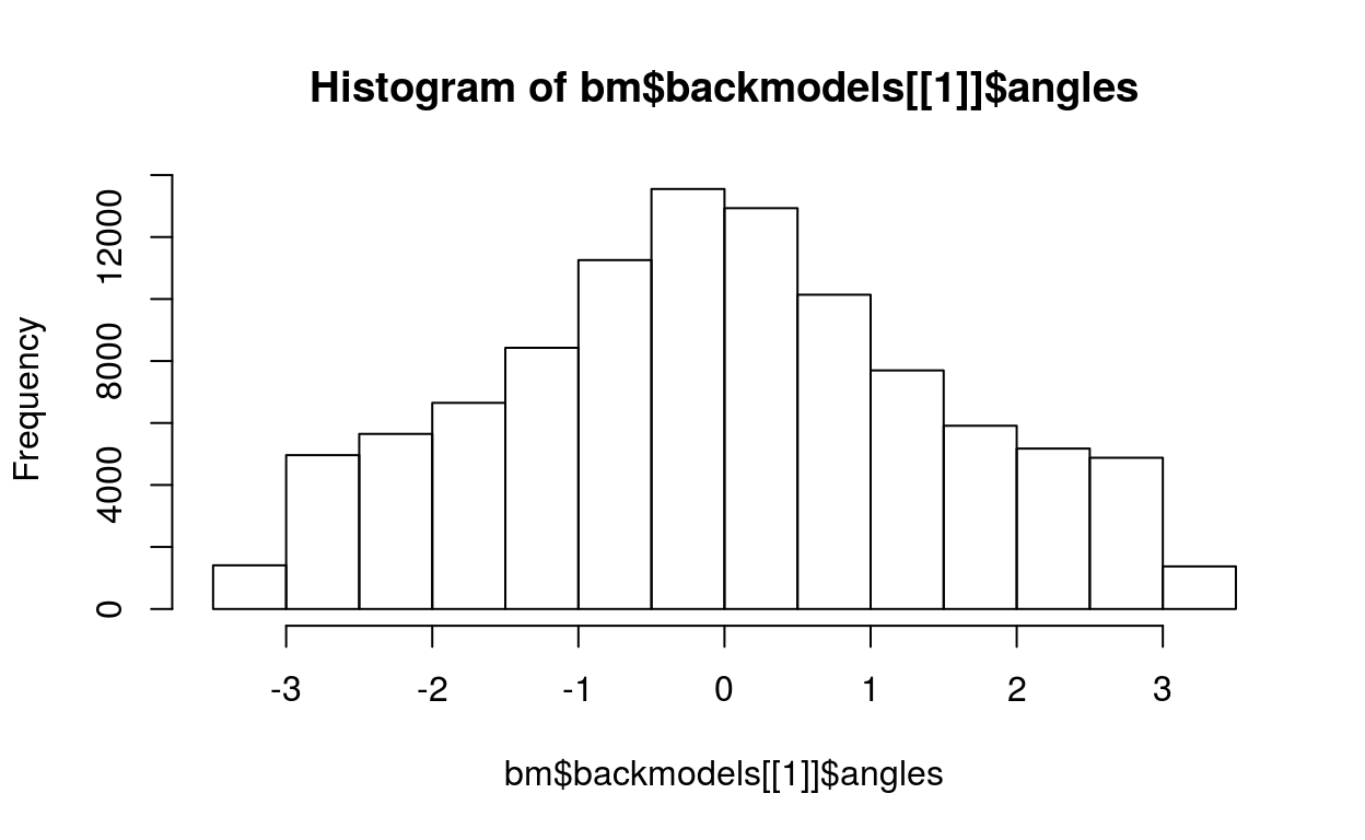

# the whole distribution (and therefore also the p-value) also depends on the mean angle
plotdata = data.frame(angle = cut(bm$backmodels[[1]]$angles, 10), z = bm$backmodels[[1]]$z)
ggplot2::ggplot(plotdata) + ggplot2::geom_violin(ggplot2::aes(angle, z))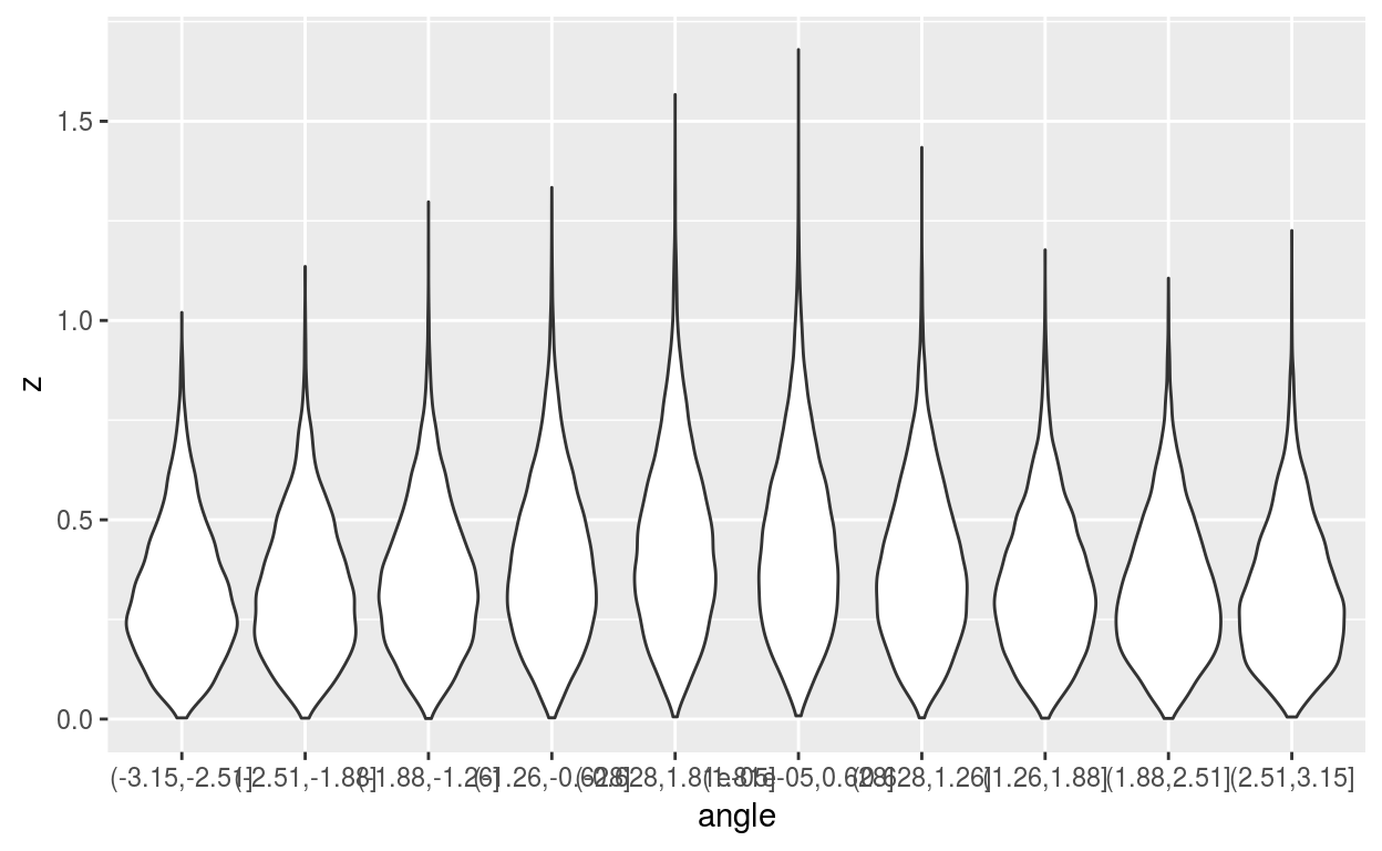

testRayleigh

Rayleigh z-test implementation

Usage

testRayleigh(angles)

Arguments

angles

Numeric vector containing angles in radians

Value

P-value of unidirectionality under the uniformity null hypothesis

Examples

testRayleigh(as.numeric(circular::rvonmises(10, circular::circular(1), 2)))

## [1] 0.004219547

testRayleigh(seq(0, 2*pi, 0.1))

## [1] 0.9995545

estimateRedundancy

Estimates the redundancy of enriched gene sets

Wrapper around the mgsa method

Usage

estimateRedundancy(scores, gsets, Gdiffexp)

Arguments

scores

Dataframe from testUnidirectionality() containing the filtered enrichment scores for every gene set

gsets

Named list containing character vectors for each gene set

Gdiffexp

Character vector of differentially expressed genes

Value

Numeric vector containing for every gene set (in the same order the scores dataframe) its relevance compared with other gene sets, higher is better

Examples

Eoi = matrix(rnorm(1000*3, sd=0.5), 1000, 3, dimnames=list(1:1000, c(1,2,3)))
Eoi[1:100,1] = Eoi[1:100,1] + 4 # the first 100 genes are more upregulated in the first condition
barycoords = transformBarycentric(Eoi)
Gdiffexp = (1:1000)[barycoords$r > 1]

gsets = list(a=1:50, b=c(1:50, 100:110), c=200:500) # a and b are redundant, but a is stronger enriched
scores = testUnidirectionality(barycoords, gsets, Gdiffexp=(1:1000)[barycoords$r > 1])
scores$redundancy = estimateRedundancy(scores, gsets, Gdiffexp)
scores[scores$gsetid == "a", "redundancy"] > scores[scores$gsetid == "b", "redundancy"]

## [1] TRUE

testEnrichment

Simple fisher’s exact test for enrichment in a given set of genes of interest (Goi)

Usage

testEnrichment(Goi, gsets, background, minknown = 2, mindiffexp = 2, maxknown = 500)

Arguments

Goi

character vector containing the genes tested for enrichment

gsets

List of character vectors, each containing a set of genes (gene identifiers)

background

character vector containing background gene identifiers

minknown

Minimal number of genes within a gene set for it to be considered for enrichment

mindiffexp

Minimal number of genes differentially expressed within a gene set for it to be considered for enrichment

maxknown

Maximal number of genes within a gene set for it to be considered for enrichment

Value

Dataframe containing for every gene set which passed the filtering:

• p-value of enrichment
• q-value of enrichment (p-value corrected for multiple testing)
• estimated odds score of enrichment, how much more likely is a given gene set to be part of

Examples

Goi = 1:50
gsets = list(a= 20:70, b = 45:80)
background = 1:100
testEnrichment(Goi, gsets, background)

##         pval      odds found gsetid       qval
## 1 0.02246197 2.4248312    31      a 0.04492393
## 2 0.99999997 0.0934603     6      b 0.99999997

testLocality

Test local upregulation

Tests for local upregulation locally in certain directions

Usage

testLocality(Goi, Gdiffexp, angles, deltangle = pi/24, bandwidth = pi/3)

Arguments

Goi

Gene set for which to test enrichment

Gdiffexp

Differentially expressed genes

angles

Numeric vector with angles of all genes or a dataframe as returned by transformBarycentric

deltangle

Stepsize of angles

bandwidth

Bandwidth of angles

Value

Corrected p-values for enrichment around every angle

Examples

Eoi = matrix(rnorm(1000*3, sd=0.5), 1000, 3, dimnames=list(1:1000, c(1,2,3)))
Eoi[1:100,1] = Eoi[1:100,1] + 4 # the first 100 genes are more upregulated in the first condition
barycoords = transformBarycentric(Eoi)

Goi = 1:50
qvals = testLocality(Goi, Gdiffexp=(1:1000)[barycoords$r > 1], barycoords)
plot(attr(qvals, "anglesoi"), qvals)

vandelaar

Expression dataset from van de Laar et al. 2016

This dataset contains, among others, gene expression data from the three main macrophage progenitor populations in mice. Note that due to size restrictions of Bioconductor, half of non-differentially expressed genes are not included in the dataset.

Usage

vandelaar

Format

An object of class ExpressionSet with 11679 rows and 24 columns.

Source

https://www.ncbi.nlm.nih.gov/geo/query/acc.cgi?acc=GSE76999

Value

ExpressionSet with 11679 genes and 24 samples.