Expression preprocessing

In this vignette we illustrate the triwise package using expression data from the three main cell populations contributing to adult tissue resident macrophages in mice (yolk-sac macrophages, fetal liver monocytes and bone marrow monocytes) from this study (van de Laar et al. 2016).

library(triwise)
library(limma)
library(Biobase)
data(vandelaar)

This dataset contains log2 gene expression values from, among others, the three progenitors (YS_MF, FL_mono and BM_mono) as an ExpressionSet object, each with four biological replicates (samples). We first filter this dataset on only those samples in which we are interested (Eoi_replicates) and then calculate the average expression in the three biological conditions (Eoi).

Eoi_replicates <- vandelaar[, phenoData(vandelaar)$celltype %in% c("BM_mono", "FL_mono", "YS_MF")]
dim(Eoi_replicates)

Features  Samples 
   11679       12 

Eoi <- limma::avearrays(Eoi_replicates, phenoData(Eoi_replicates)$celltype)
Eoi = Eoi[,c("YS_MF", "FL_mono", "BM_mono")]
dim(Eoi)

[1] 11679     3

colnames(Eoi)

[1] "YS_MF"   "FL_mono" "BM_mono"

Plotting gene expression of three conditions

We now transform this gene expression matrix to barycentric coordinates. This transformation will reduce the dimensionality of the gene expression data by one, and only retain the information of expression changes between samples.

barycoords = transformBarycentric(Eoi)
str(barycoords)

'data.frame':   11679 obs. of  4 variables:
 $ x    : num  -0.3455 -0.0839 -0.1047 -0.0239 -0.153 ...
 $ y    : num  0.1199 -0.0439 -0.1069 0.1556 0.1784 ...
 $ angle: num  2.81 -2.66 -2.35 1.72 2.28 ...
 $ r    : num  0.3657 0.0947 0.1496 0.1574 0.235 ...
 - attr(*, "conditions")= chr  "YS_MF" "FL_mono" "BM_mono"

These barycentric coordinates can then be plotted in a 2D dotplot. In this plot every gene is represented by a single dot. The direction of a dot indicates in which condition(s) the gene is upregulated, while the distance from the origin represents the strength of upregulation (in the same order of magnitude as a log fold-change). Genes with the same expression in all three samples will all lie close to eachother in the center, regardless of the height of their absolute expression values. Points lying on a hexagon gridline all have the same maximal fold-change between any two pairwise comparisons.

plotDotplot(barycoords)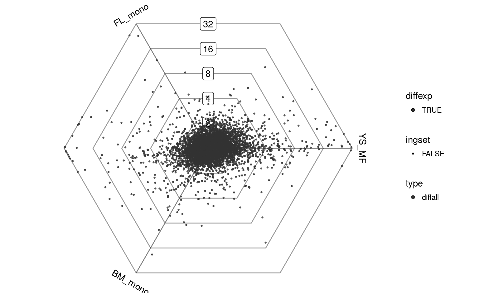

Overall, the main difference in expression seems to be between the two monocytes (FL_mono and BM_mono) and the yolk sac macrophage (YS_MF). However, one can also appreciate the number of genes which are specifically upregulated in one of the two monocytes, or are shared between one monocyte and the yolk sac macrophage.

We can use limma to determine which genes are differentially expressed in any of the three conditions and visualize these genes on the dotplot. The differentially expressed genes are shown in black.

design = as(phenoData(Eoi_replicates), "data.frame")
design$celltype = factor(as.character(design$celltype))
design <- model.matrix(~0+celltype, design)
fit <- lmFit(Eoi_replicates, design)
fit = contrasts.fit(fit, matrix(c(1, -1, 0, 0, 1, -1, 1, 0, -1), ncol=3))
fit = eBayes(fit)

top = topTable(fit, p.value=0.05, lfc=1, number=Inf, sort.by = "none")
Gdiffexp = rownames(top)

plotDotplot(barycoords, Gdiffexp)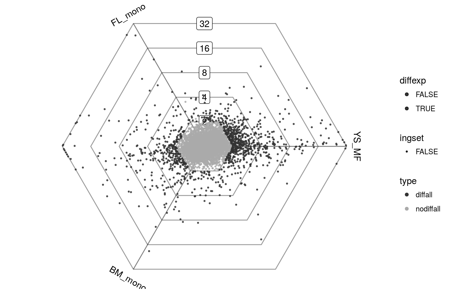

We can also plot this as a rose plot, a polar histogram showing the directional distribution of the differentially expressed genes. When plotting all genes in this way it can give you a sense of the main expression changes between populations. As we will see later, it can also be used to visualize individual sets of genes.

plotRoseplot(barycoords, Gdiffexp, relative = F)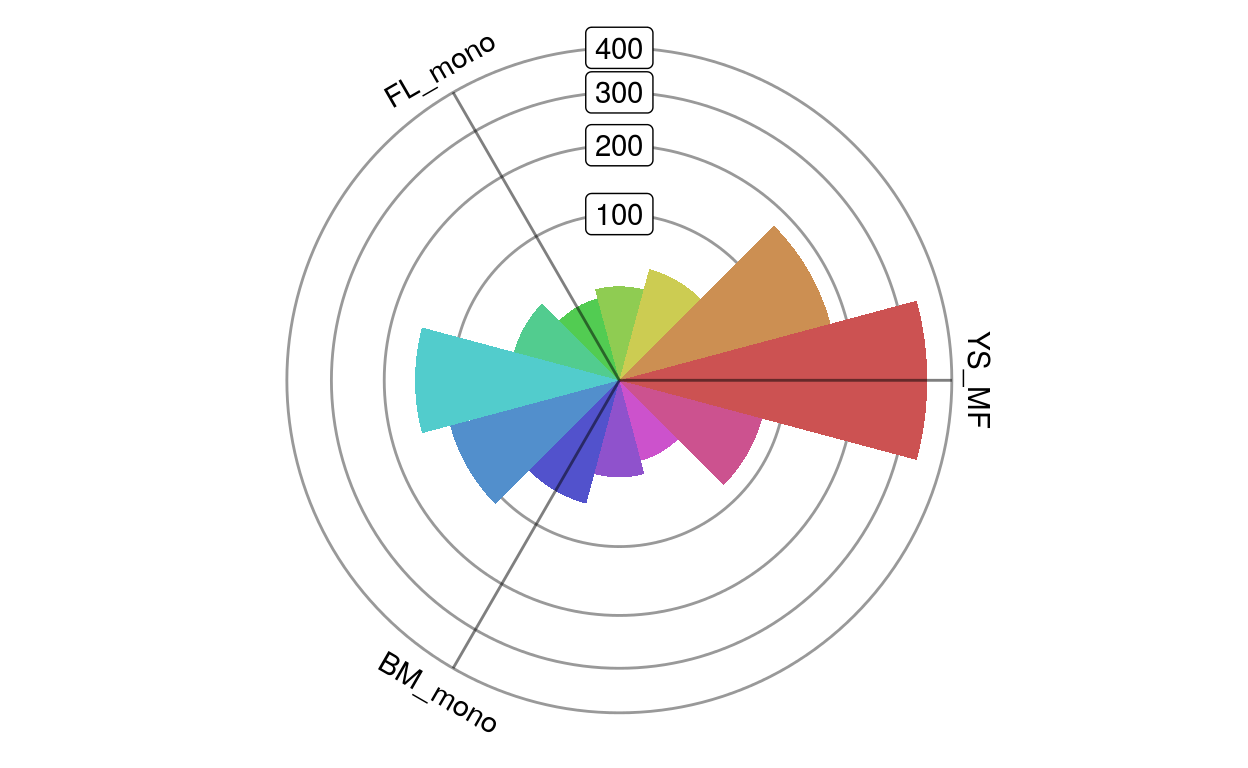

The dotplots can also be explored interactively using an htmlwidget. These can be saved as standalone html pages using saveWidget(dotplot, file="dotplot.html"). When using RStudio, the GUI can also be used to export the plot as a bitmap png image. Within the widget, genes of interest can be selected to show their labels on the outside of the plot.

dotplot = interactiveDotplot(Eoi, Gdiffexp, Glabels = featureData(vandelaar)$symbol, Goi=dplyr::top_n(top, 25, -adj.P.Val)$entrez)
dotplot

Analyzing functional diversity of three biological conditions

One of the nice applications of analyzing three conditions at a time is that it allows you to find (partly) shared functional gene sets up or downregulated in one or two conditions. This is illustrated here for genes annotated with a particular function through GO.

We first extract the relevant information of the genes sets from the Bioconductor annotation packages. We also filter the gene sets for genes within the expression datasets.

library(org.Mm.eg.db)
library(GO.db)
library(dplyr)
gsets = AnnotationDbi::as.list(org.Mm.egGO2ALLEGS)
gsets = sapply(gsets, function(gset) intersect(rownames(Eoi), unique(as.character(gset))))
gsetindex = dplyr::bind_rows(lapply(AnnotationDbi::as.list(GOTERM[names(gsets)]), function(goinfo) {
  tibble(name=Term(goinfo), definition=Definition(goinfo), ontology=Ontology(goinfo), gsetid = GOID(goinfo))
}))
gsets = gsets[gsetindex %>% filter(ontology == "BP") %>% .$gsetid]

We now test whether a gene set is specifically upregulated in a particular direction. This can be run in parallel using the mc.cores parameters (not available on Windows).

scores = testUnidirectionality(barycoords, gsets, Gdiffexp, statistic = "rank", mc.cores = 8, nsamples=1e+6)
scores = left_join(scores, gsetindex, by="gsetid") %>% filter(qval < 0.05) %>% arrange(qval, z)

Results from GO enrichment tend to include a lot of redundancy because of large overlaps between individual GO terms. To improve interpretability, Triwise therefore uses the “model-based gene set analysis” method (Bauer, Gagneur, and Robinson 2010) which selects those gene sets optimally explaining the differentially expressed genes in the dataset.

scores = scores[(scores$qval < 0.05) & (scores$z > 0.15), ]
scores$redundancy = estimateRedundancy(scores, gsets, Gdiffexp)

Non-redundant gene sets are upregulated in different directions.

plotPvalplot(scores %>% top_n(20, redundancy), colnames(Eoi))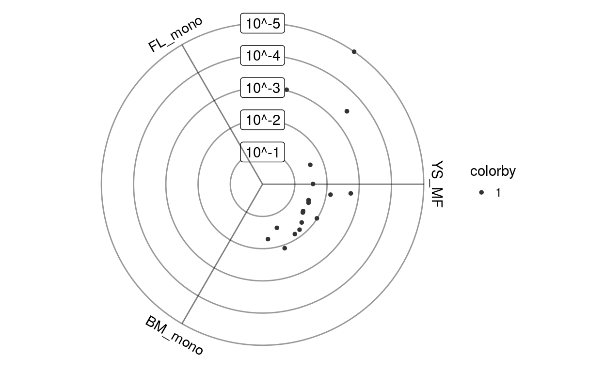

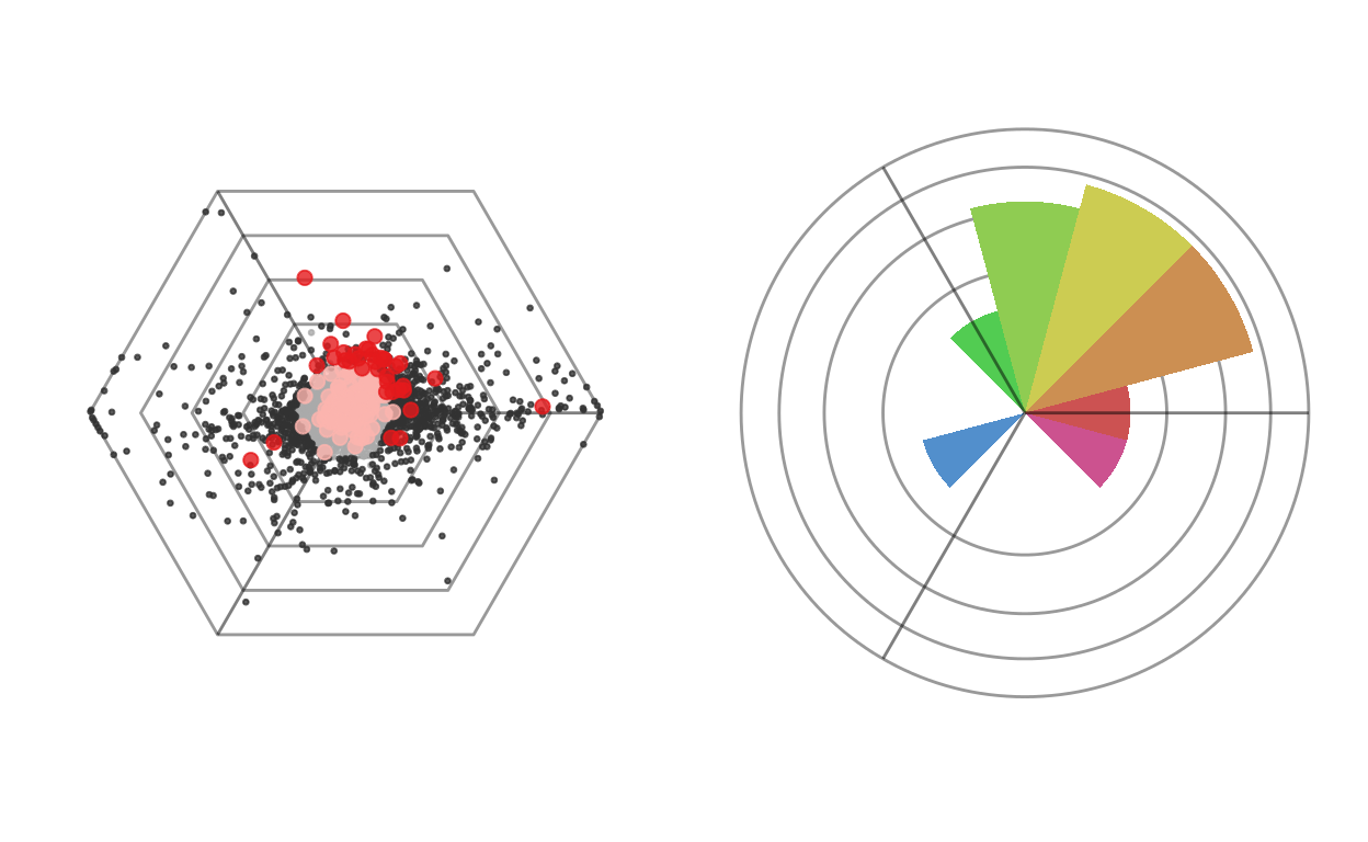
Individual gene sets can then again be plotted on a dotplot.

gsetid = gsetindex$gsetid[gsetindex$name == "DNA replication"]
cowplot::plot_grid(
  plotDotplot(barycoords, Gdiffexp, Goi=gsets[[gsetid]], showlabels = F, Coi=c("")) + ggplot2::theme(legend.position = "none"), 
  plotRoseplot(barycoords, Gdiffexp, Goi=gsets[[gsetid]], relative = T, showlabels = F, Coi=c(""))
)

We can also have a look at the top enriched gene sets.

plots = lapply(scores %>% top_n(8, redundancy) %>% .$gsetid, function(gsetid) {
  plotDotplot(barycoords, Gdiffexp, Goi=gsets[[gsetid]], showlabels = F) + 
    ggplot2::theme(legend.position = "none") + 
    ggplot2::ggtitle(gsetindex$name[match(gsetid, gsetindex$gsetid)] %>% strwrap(40) %>% paste(collapse="\n")) + 
    ggplot2::theme(axis.text=ggplot2::element_text(size=14), plot.title=ggplot2::element_text(size=8,face="bold"))
})

cowplot::plot_grid(plotlist=plots, ncol=4)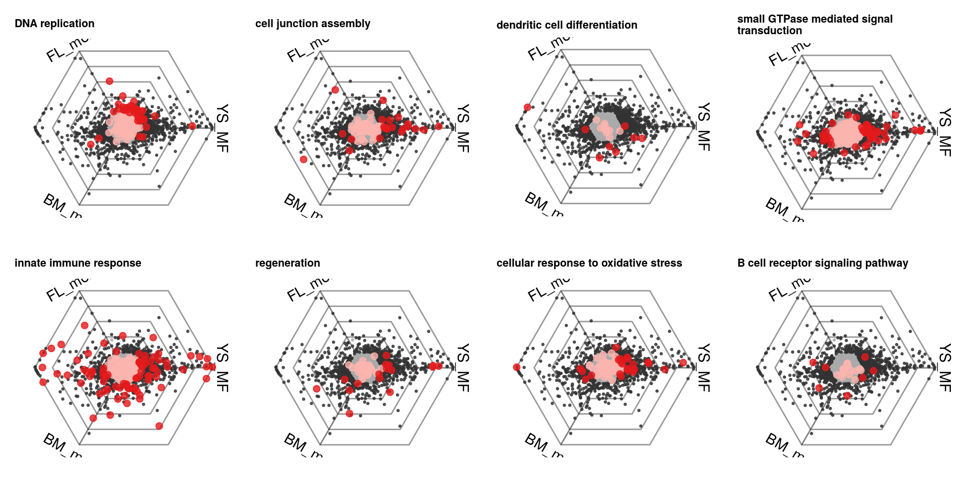

plots = lapply(scores %>% top_n(8, redundancy) %>% .$gsetid, function(gsetid) {
  plotRoseplot(barycoords, Gdiffexp, Goi=gsets[[gsetid]], showlabels = F) + 
    ggplot2::theme(legend.position = "none") + 
    ggplot2::ggtitle(gsetindex$name[match(gsetid, gsetindex$gsetid)] %>% strwrap(40) %>% paste(collapse="\n")) + 
    ggplot2::theme(axis.text=ggplot2::element_text(size=14), plot.title=ggplot2::element_text(size=8,face="bold"))
})

cowplot::plot_grid(plotlist=plots, ncol=4)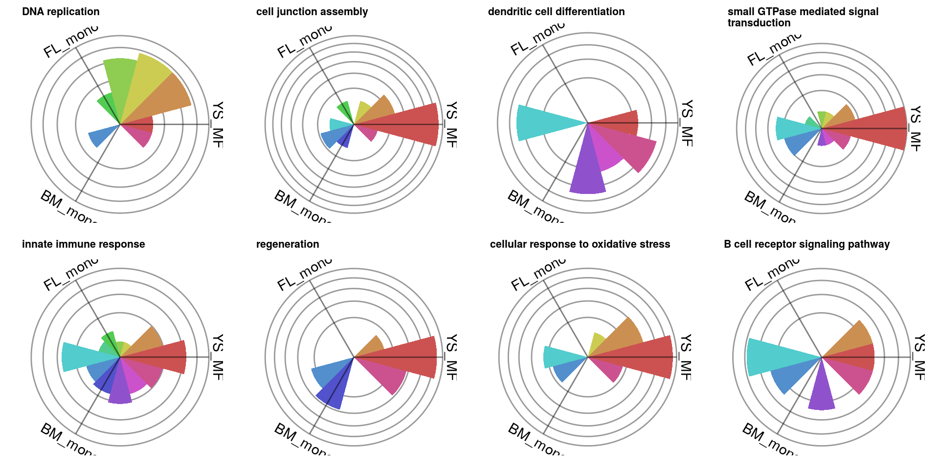

It is for example clear that genes related to cell cycle initiation are upregulated in both monocytes, while genes associated with viral responses are downregulated in the FL monocyte.

plotDotplot(barycoords, Gdiffexp, gsets[scores %>% top_n(3, redundancy) %>% .$gsetid])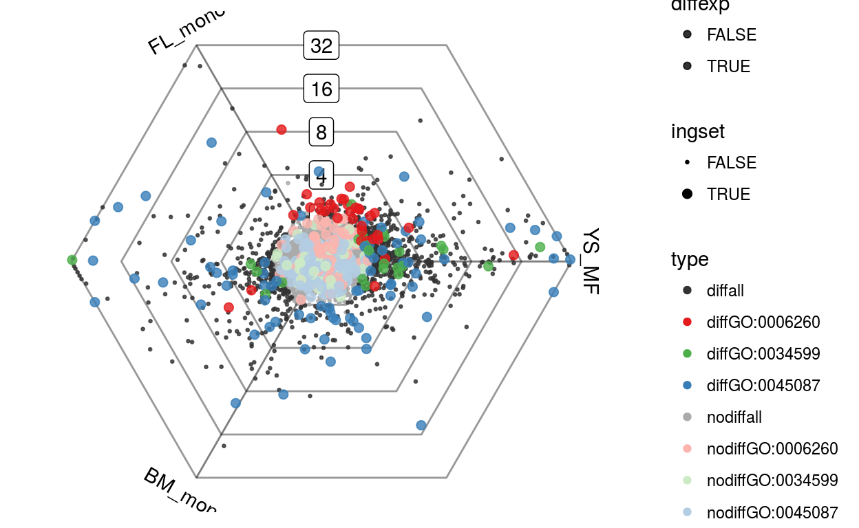

Visualizing changes in differential expression between pairs of biological conditions

We can also visualize what happens to the expression differences when these three progenitor cells are transferred to the lungs (leading to them becoming alveolar macrophages).

We first select those genes which are differentially expressed both between the original progenitor cells and between the transferred cells.

diffexp <- function(E_replicates, c1, c2) {
  design = as(phenoData(E_replicates)[phenoData(E_replicates)$celltype %in% c(c1,c2),], "data.frame")
  design$celltype = factor(as.character(design$celltype), levels=c(c2, c1)) # relevel so that contrast is in the right direction
  designmat = model.matrix(~0+celltype, design)
  colnames(designmat) <- c("A","B")
  fit <- lmFit(E_replicates[,rownames(design)[design$celltype %in% c(c1,c2)]],designmat)
  contrastmat <- makeContrasts("B-A", levels=designmat)
  fit = contrasts.fit(fit, contrastmat)
  fit = eBayes(fit)
  top = topTable(fit, p.value=0.05, lfc=1, number=Inf, sort.by = "none")
  
  list(up = rownames(top)[top$logFC > 1], down=rownames(top)[top$logFC < -1])
}

Goi = list(
  YSup = intersect(diffexp(vandelaar, "YS_MF_AMF", "FL_mono_AMF")$up, diffexp(vandelaar, "YS_MF_AMF", "BM_mono_AMF")$up),
  YSdown = intersect(diffexp(vandelaar, "YS_MF_AMF", "FL_mono_AMF")$down, diffexp(vandelaar, "YS_MF_AMF", "BM_mono_AMF")$down),
  FLup = intersect(diffexp(vandelaar, "FL_mono_AMF", "BM_mono_AMF")$up, diffexp(vandelaar, "FL_mono_AMF", "YS_MF_AMF")$up),
  FLdown = intersect(diffexp(vandelaar, "FL_mono_AMF", "BM_mono_AMF")$down, diffexp(vandelaar, "FL_mono_AMF", "YS_MF_AMF")$down),
  BMup = intersect(diffexp(vandelaar, "BM_mono_AMF", "FL_mono_AMF")$up, diffexp(vandelaar, "BM_mono_AMF", "YS_MF_AMF")$up),
  BMdown = intersect(diffexp(vandelaar, "BM_mono_AMF", "FL_mono_AMF")$down, diffexp(vandelaar, "BM_mono_AMF", "YS_MF_AMF")$down)
)
Goi = Filter(function(x) length(x>0), Goi)

We can now supply a second barycoords to the plotDotplot function. It is clear that the direction of upregulation of certain genes remains stable before and after transfer to the lungs. For other genes the specificity changes.

Eoi2_replicates <- vandelaar[, phenoData(vandelaar)$celltype %in% c("YS_MF_AMF", "FL_mono_AMF", "BM_mono_AMF")]
Eoi2 <- limma::avearrays(Eoi2_replicates, phenoData(Eoi2_replicates)$celltype)
Eoi2 = Eoi2[,c("YS_MF_AMF", "FL_mono_AMF", "BM_mono_AMF")]
barycoords2 <- transformBarycentric(Eoi2)

plotDotplot(barycoords, unlist(Goi), Goi=Goi, barycoords2 = barycoords2) + ggplot2::theme(legend.position="none")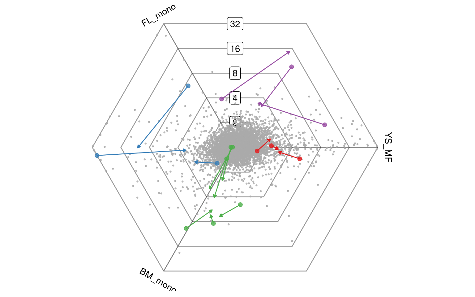

Session info

sessionInfo()

R version 3.3.2 (2016-10-31)
Platform: x86_64-pc-linux-gnu (64-bit)
Running under: Ubuntu 14.04.5 LTS

locale:
 [1] LC_CTYPE=en_US.UTF-8       LC_NUMERIC=C              
 [3] LC_TIME=en_US.UTF-8        LC_COLLATE=en_US.UTF-8    
 [5] LC_MONETARY=de_BE.UTF-8    LC_MESSAGES=en_US.UTF-8   
 [7] LC_PAPER=de_BE.UTF-8       LC_NAME=C                 
 [9] LC_ADDRESS=C               LC_TELEPHONE=C            
[11] LC_MEASUREMENT=de_BE.UTF-8 LC_IDENTIFICATION=C       

attached base packages:
[1] stats4    parallel  stats     graphics  grDevices utils     datasets 
[8] methods   base     

other attached packages:
 [1] dplyr_0.5.0          GO.db_3.3.0          org.Mm.eg.db_3.3.0  
 [4] AnnotationDbi_1.34.0 IRanges_2.6.0        S4Vectors_0.10.0    
 [7] limma_3.28.6         triwise_0.99.0       Biobase_2.32.0      
[10] BiocGenerics_0.18.0 

loaded via a namespace (and not attached):
 [1] Rcpp_0.12.8          mgsa_1.20.0          BiocInstaller_1.24.0
 [4] RColorBrewer_1.1-2   git2r_0.16.0         circular_0.4-7      
 [7] plyr_1.8.4           tools_3.3.2          highlight_0.4.7     
[10] boot_1.3-18          digest_0.6.10        RSQLite_1.0.0       
[13] jsonlite_1.1         evaluate_0.10        memoise_1.0.0       
[16] tibble_1.2           gtable_0.2.0         DBI_0.5-1           
[19] yaml_2.1.14          withr_1.0.2          stringr_1.1.0       
[22] knitr_1.15.1         htmlwidgets_0.8      packagedocs_0.4.0   
[25] devtools_1.12.0      cowplot_0.7.0        grid_3.3.2          
[28] R6_2.2.0             rmarkdown_1.1        ggplot2_2.2.0       
[31] magrittr_1.5         whisker_0.3-2        scales_0.4.1        
[34] htmltools_0.3.5      MASS_7.3-45          lazyrmd_0.2.0       
[37] assertthat_0.1       colorspace_1.3-1     labeling_0.3        
[40] stringi_1.1.2        lazyeval_0.2.0       munsell_0.4.3